Arithmetic derivatives and outsmarting the heat death of the unvierse
Question statement
(…and conventional introductory ramble)
So a couple days about a week ago, just as I was putting in some finishing touches to my previous blog post (and the blog itself), my roommate asked me for some programming help. He told me he wanted to filter out unique elements of an array along with their count as a single object. Being the kind and benevolent soul that I am, I helped him with it. But at the same time being a nosy little thing, I wondered why this man needed to filter arrays in the middle of the day – and so I asked him, and thus began a three day journey filled with numerous dead-ends, random insights, unexpected discoveries (and hours upon hours of wasted runtime) all in the hopes of trying to solve this very cool problem. Here is the set up.
The arithmetic derivative is defined by
- $p’ = 1$ when p is a prime number
- Given positive integers $a$ and $b$ we define $(ab)’ = a’b + ab’$
For example, $20’ = (2^2 \cdot 5)’ = (2^2)’\cdot 5 + 2^2 = (2 + 2)\cdot 5 + 4 = 24$.
The question now seeks to find the following sum
$$\sum_{k=2}^{5\times 10^{15}} \mathrm{gcd}(k,k’)$$
Source: Project Euler, problem 484
I would be lying if I said the first thought that crossed my mind after reading this problem was not “Oh, this seems like a cool problem to put in the blog!”. To be honest these are the kind of problems that motivated me to have this series going in the first place.
Before I get into the nitty-gritty details of this problem, here is a disclaimer:
$$\underline{\textbf{ I am not going to be posting the full solution to this problem below. }}$$
The reason for this is best explained in the about page of Project Euler.
Q: I learned so much solving problem XXX, so is it okay to publish my solution elsewhere?
A: It appears that you have answered your own question. There is nothing quite like that “Aha!” moment when you finally beat a problem which you have been working on for some time. It is often through the best of intentions in wishing to share our insights so that others can enjoy that moment too. Sadly, that will rarely be the case for your readers. Real learning is an active process and seeing how it is done is a long way from experiencing that epiphany of discovery. Please do not deny others what you have so richly valued yourself.
With that out of the way, what I will do in this post though is go over some of the hints discussed in this discussion forum and give more of a background and context to them. If you would like to challenge yourself without my help, I welcome you to close the blog post right now, and go on your own three-day (or shorter/longer) journey.
For those who chose to continue with the post, here’s a run down of what we will discuss. We start by reviewing some of my naive initial attempts and discuss why they are utter trash. Then we look for some mathematical short-cuts that will help the code terminate before the end of human civilization two hundred million years from now (if we don’t already kill ourselves by then). In the section following that, we will discuss good coding strategies that might come very much in handy in bringing down the time complexity of the problem. Towards the end of the post, I will also summarize all the theory was discussed in the post from perspective of this problem, and in doing so, provide a (hopefully identifiable) skeleton of a solution.
So buckle up, here we go!
Et-tu Brute Force
Now if you are anything like me (aka. commutative algebraist), you see a problem like this and you start considering the most general possible case and outlining an algorithm based on that. So let us do just that. Start with a random natural number $n$ and since it is possible to uniquely factor any natural number as a product of primes, let us say $n = p_1^{\alpha_1}p_2^{\alpha_2}\dots p_n^{\alpha_n}$. Then we compute $n’$ using the product rule given in the problem
$$n’ = (\alpha_1 p_1^{\alpha_1 - 1}p_2^{\alpha_2}\dots p_n^{\alpha_n}) + \dots + (\alpha_n p_1^{\alpha_1}p_2^{\alpha_2}\dots p_n^{\alpha_n - 1})$$
looking at it closely, it is easy to simplify that as
$$n’ = \sum_{i=1}^n \alpha_i \frac{n}{p_i}$$
Now, all that is left to do is calculate is $\mathrm{gcd}(n,n’)$. So we have
$$\mathrm{gcd}(n,n’) = \mathrm{gcd}\left(\prod_{i=1}^n p_i^{\alpha_i}, \sum_{i=1}^n \frac{\alpha_i}{p_i}n \right) = \left[\prod_{i=1}^n p_i^{\alpha_i-1}\right]\mathrm{gcd}\left(\prod_{i=1}^n p_i, \sum_{i=1}^n \frac{\alpha_i}{p_i} n\right)$$
Notice that we can’t factor the $n$ out of the $\mathrm{gcd}$ term because we don’t know if the sum $\sum_{i=1}^n \frac{\alpha_i}{p_i} \in \mathbb{Z}$.
So the approach is clear. Given an upper bound $L$, we simply have to consider every natural number between $2$ and $L$, factorize it along with its corresponding the exponents, use that to compute the $\mathrm{gcd}(n,n’)$ as shown above and add it all up!
Easy, right? …right?
Uh, well – not really (but we’ll get there). Let’s try and understand why.
First of all, we need a way to factorize any given number into its constituent primes and identify their corresponding exponents. But this is not terribly hard once you sit down and really think about it for maybe fifteen to twenty minutes.
Here’s a nice little function that would do it for you.
1 | def primeFactors(n): |
The code isn’t optimized, but it runs quite fast. It can comfortably factorize $12312234873493412134$ in about 3 seconds (in interpreted python). Once this is done, the rest of the code falls into place quite nicely. I’m not going to bore you with the details of implementation of the algorithm 1. Here is why it is bad:
I ran the algorithm for smaller values of $L$ fairly successfully, and then I started to progressively increase the value of $L$ to see how well it performed as $L$ went up. I also made the effort to tabulate the run-time for each $L$ value. Below I’ve reproduced a plot I made comparing the run-time of this algorithm against $\log_{10}(L)$ (this was done mainly to squish down the $x-$axis to a realistic scale).
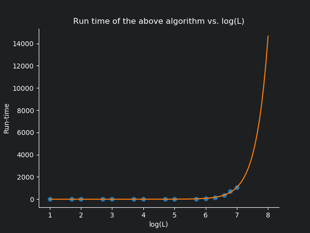
Looking at the graph, it is pretty apparent that the runtime grows exponentially against $\log(L)$!. As a matter of fact, the equation of the orange curve is
$$y = 0.0085e^{2.6123\log_{10}(x)-2.5020}-5.1564$$
Therefore, setting $x = 5 \times 10^{15}$ we get $y = 4.50125 \times 10^{14}$ seconds.
Just to sort of picture that, running on a single computer, it would take about $14274.17$ millenniums for the code to finish running. We could also parallelize it over a million computers (good luck getting your hands on them), and you can bring the run time down to about $14.27$ years. According to this website, we can estimate that there are about four billion personal computers being used world-wide today (I’m assuming the military grade tech is kind of out of our reach). Parallelizing this algorithm across every single computer in the world that is active and running right now, the program would terminate after running for $1.3$ days 2
So we can agree that this is going nowhere (honestly I only wrote this entire section to engage in these fun hypotheticals).
Can you crunch those numbers again?
-Micheal Scott. Founder, Micheal Scott paper company
So we are back at our drawing board again. This time around, armed with some idea of how our previous algorithm fits together – we are going to approach it in a more ground-up way. Lets not take any arbitrary number $n$, and instead let $n=p^\alpha$ where $\alpha \geq 1$. Since (integer-)exponents are just glorified products, we readily see that the power rule of normal derivatives applies to arithmetic derivatives as well! So
$$n’ = \alpha p^{\alpha - 1}$$
This is quite cool! Moreover, we can also get $$\mathrm{gcd}(n,n’) = p^{\alpha - 1} \mathrm{gcd}(\alpha, p)$$
Now, in the case that $\alpha$ and $p$ are coprime, it is straightforward that $\mathrm{gcd}(\alpha, p) = 1$ and in the case where $p|\alpha$, we have $\mathrm{gcd}(\alpha, p) = p$ (to make it a bit more apparent, $\alpha$ can be composite. So write it’s prime factorization and consider both cases). So this gives us a pretty nice formula. Given $n = p^\alpha$ with $p$ prime and $\alpha \geq 1$,
$$g(n) = \mathrm{gcd}(n,n’) = \begin{cases} p^{\alpha}; & p|\alpha \\ p^{\alpha-1}; & p\not|\alpha \end{cases} = \begin{cases} n; & p|\alpha \\ \frac{n}{p}; & p\not|\alpha \end{cases}$$
So,
Fact 1: $g$ is nice for prime powers.
This is actually quite good, we are making progress, we have probably cut down so much of the computational complexity. But we can do better. Lets up the difficulty a notch. What if $n = p^{\alpha}n_1$ where $n_1 \in \mathbb{Z}$ such that it is coprime to $p$? Well, in this case, $$g(n) = \mathrm{gcd}(n,n’) = \mathrm{gcd}(p^{\alpha}n_1, \alpha p^{\alpha-1}n_1 + p^{\alpha}n_1’)$$
Which honestly looks like a mess. So we naturally go to wikipedia and look at GCD properties (looking for some distributive-esque properties). We discover that the following two serve very useful
- $\mathrm{gcd}(a+mb,b) = \mathrm{gcd}(a,b)$
- $\mathrm{gcd}(da + db) = d \cdot \mathrm{gcd}(a,b)$
In our case, we can simplify that expression as follows.
$$\mathrm{gcd}(p^{\alpha}n_1, \alpha p^{\alpha-1}n_1 + p^{\alpha}n_1’) = \left[p^{\alpha -1}\mathrm{gcd}(p,\alpha)\right]\mathrm{gcd}\left(n_1, \frac{\alpha}{\mathrm{gcd}(p,\alpha)}n_1 + n_1’\right)$$
where we used the second property of GCD listed above. To explain it a bit further, obviously $p^{\alpha -1}$ is a common factor. But there is more! In the case of $p|\alpha$ we get another factor of $p$ (both among $p$ and $\alpha$) that we can factor out (and in case $p\not| \alpha$, $\mathrm{gcd}(p,\alpha) = 1$ anyway. So it doesn’t hurt to factor that out.)
Now, we use property $2$ in reverse for $\left[p^{\alpha -1}\mathrm{gcd}(p,\alpha)\right]$ to see $$\left[p^{\alpha -1}\mathrm{gcd}(p,\alpha)\right] = \mathrm{gcd}(p^\alpha, \alpha p^{\alpha -1 }) = g(p^{\alpha})$$
We use first property in $\mathrm{gcd}\left(n_1, \frac{\alpha}{\mathrm{gcd}(p,\alpha)}n_1 + n_1’\right)$ to see that
$$\mathrm{gcd}\left(n_1, \frac{\alpha}{\mathrm{gcd}(p,\alpha)}n_1 + n_1’\right) = \mathrm{gcd}(n_1, n_1’) = g(n_1)$$
So putting everything together, we have
$$g(n) = g(p^\alpha n_1) = g(p^{\alpha})g(n_1)$$
This tells us that $g$ is a multiplicative function! This means we only have to focus on prime numbers alone (and not necessarily all numbers from $2 \rightarrow L$).
So,
Fact 2: Fact 1 just got 200 times nicer; because given $n=\prod_{i=1}^r p_i^{\alpha_i}$,$$g(n) = \prod_{i=1}^r g(p_i^{\alpha_i})$$
This is really good! Now the game plan is to find every prime under $n$ and then compute the required sum from there using the multiplicative property. But here even with the most optimized code, our time complexity is still $\mathcal{O}(n)$ because we have to construct every number under $n$ at least once. I welcome you to write a script with these new modifications and run it to see why $\mathcal{O}(n)$ is still very slow for an average computer. Now going back to the plot I made with the run times for my initial naive attempt, it looks like $10^{15}$ is unattainable by realistic standards, but $10^{7}$ sounds doable. So maybe, if we could write an algorithm that is $\mathcal{O}(\sqrt{n})$, we might just be able to solve this.
But this means, we have to somehow cut the number of computations down to its geometric half. Let us go back and see if there is some other nice property that we have missed so far…
Going back to the case where $n=p^e$, what happens when $e=1$, well $n’ = 1$, and so $g(n)=1$. Since $g$ is multiplicative, this means for any square free number $n$, we have $g(n) = 1$! 3. In fact, we can do even better! Notice that for any $n = p^{\alpha}n_1$ with $\alpha > 1$ and $n_1$ being square free, $g(n) = g(p^{\alpha})$.
To write this out properly as a fact, we need the following definition (to make writing a lot easier).
A positive integer $n$ is a powerful integer if we have for any prime $p$ satisfying $p|n$, we also have $p^2|n$.
That is to say, in the prime factorization of a powerful number $n$, all exponents are strictly greater than $1$
So, we can use this definition to obtain the following fact
Fact 3: for any powerful number $n_1$ and squarefree number $n_2$, $g(n_1 \cdot n_2) = g(n_1)$.
This gives us a really cool idea! If $n$ is a powerful number under $L$, for every square free number $r$ under $\left \lfloor{L/n} \right\rfloor$ we have $g(nr) = g(n)$. So we just need a way to get all the powerful numbers under $L$ and find the number of squarefree numbers under $\left \lfloor{L/n} \right\rfloor$ for any given powerful $n$.
This is because given some powerful $n$, and $t$ squarefree numbers under $\left \lfloor{L/n} \right\rfloor$, $g(n)$ is going to be added $t$ times in the final sum we are trying to calculate! So we simply calculate $g(n)$ and multiply it by $t$!
Now, the real question is, can this be achieved in $\mathcal{O}(\sqrt{n})$? The answer is, if you are careful with your code, it is possible!
First of all we need a way to enumerate all the powerful numbers under $L$. The beautiful thing about powerful numbers is that there are only about $2\sqrt{L}$ of them (see if you can understand why). With a clever way of enumerating them, you can get this process running in $\mathcal{O}(\sqrt{n})$. This clever way of enumerating them is called Dynamic programming and that’s what I’ll cover in the next section.
Now comes the issue of finding the number of square free numbers under a given number, and fortunately for us, this is not hard either! A quick search reveals this goldmine where we can find a sublinear algorithm that is $\mathcal{O}(\sqrt{n})$ as well!
Particularly, I am talking about
$$Q(n) = \sum_{d=1}^{\sqrt{n}} \mu(d)\left \lfloor{\frac{n}{d^2}} \right\rfloor$$
where $Q(n)$ equals the number of square-free numbers under $n$ and $\mu(d)$ is the Mobius function defined via.
$$\mu(d) = \begin{cases}
1 & n \text{ is square free with even number of prime factors} \\ -1 & n \text{ is square free with odd number of prime factors} \\ 0 & \text{ otherwise }
\end{cases}$$
Thus this is now our game plan:
- Use dynamic programming to obtain all powerful numbers under $L$ and their corresponding $g$-values.
- For each powerful number $n$, find the number $t$ of square-free numbers under $\left \lfloor{L/n} \right\rfloor$
- sum up $t \times g(n)$ as you go!
Now we win!
This is in-fact, how I solved the problem. It took quite a bit of time to run, but nothing very unrealistic. The total run-time of this algorithm was $68$ minutes (give or take $5$ minutes) in interpreted python.
In order to understand recursion…
(One must first understand recursion)
In this section I will give a general outline on how to turn the above game-plan into code. I highly recommend looking over this post if you have not seen dynamic (or recursive) programming before.
Since you are reading on, I am going to assume you generally know how recursion works, and the very basics of how to make recursion better via dynamic programming. Now back to our problem. We are happy that there are only about $2\sqrt{L}$ powerful numbers – but how are we going to find them? An approach would be to use something like the Sieve of Eratosthenes to generate all prime numbers under $\sqrt{L}$. In fact, as you generate the primes, you could also compute $\mu(d)$ for every $d \leq \sqrt{L}$ rather easily (when you mark multiples $rp$ of $p$ as not prime, just keep track of the number of factors $r$ and assign $\mu(rp)$ accordingly). This will help us out when we are trying to calculate the number of square-free numbers under $\left \lfloor{L/n} \right\rfloor$ for some powerful $n$.
Once the primes are generated, we run through the array of primes and to each prime $p$, we compute its successive powers until we reach $n$ such that $p^n > L$. We store these values in a 2-D grid. Say if $L=50$ the 2-D grid would look like
\begin{bmatrix} [2 & 4 & 8 & 16 & 32] \\ [3 & 9 & 27] & & \\ [5 & 25] & & & \\ [7 & 49] & & &\end{bmatrix}
Now it’s time for some dynamic programming. For the first prime $p_1$, we start with $p_1^2$ (and add it to an empty list). We check if $p_1^2\cdot p_2 > L$, if it is, there is no point in continuing at all. If on the other hand $p_1^2 \cdot p_2 \leq L$, then we check if $p_1^2p_2^2 \leq L$. If it is, we have a powerful number and we add it to our list of powerful numbers (If not we proceed to $p_1^2p_3$ and then if it is $\leq L$ we go check $p_1^2p_3^2$ and so on). In the case $p_1^2p_2^2$ was a valid powerful number, we call the function again, but this time, with $p_1^2p_2^2$ as an input and we check if $p_1^2p_2^2p_3 \leq L$, if it is, we check $p_1^2p_2^2p_3^2$ and continue like that. Of course every time we find a powerful number, we add it’s $g$ value to a different list as they will serve useful while we are computing the final sum.
To exemplify this, let us consider the case $L=50$. Let pow = [1]. We start with $p_1 = 2$, so pow = [1,4] for now. Now we check if $4\cdot 3 \leq 50$, which it is. Now, we check $4\cdot 3^2 = 36 \leq L$ so we get another powerful number that we append to pow. So pow = [1,4,36]. Now we call the main function with 36 to check if $36 \cdot 5 \leq L$, which it isn’t. So we stop and return the list to the previous recursion where it is stored under a new variable new_pow. pow however in this level of recursion is still pow = [1, 4] and now we check if $4 \cdot 3^3 \leq L$, which it isn’t so we stop proceeding down the 2-D grid and just return new_pow to the main level where pow = [1]. Now we proceed to 8 and append it to pow and check if $8 \cdot 3 \leq L$, which it is. Now we check $8 \cdot 3^2 > L$ so we ignore the rest of the second row. We move on to the third row to see if $8\cdot 5 \leq L$ which it is, and we check $8 \cdot 25 > 50$ so we ignore the rest of the third row. And for the fourth row, $8\cdot 7 > L$, so we don’t even bother going down that row. And that’s it for $8$, so we return pow = [1,8] to the previous recursion, where the new_pow is updated with the new value $8$. Then we proceed onto $16$ so on… By the end of the process we would have enumerated all the powerful numbers!
This process looks like it is doing much more than $\sqrt{L}$ but as the primes get bigger, their corresponding powers that fit under $L$ gets smaller and smaller, and after a while we will only have to do one extra check per-prime, and the process is more or less $\mathcal{O}(\sqrt{L})$.
We have already computed all the $\mu$ values while the primes were generated using the sieve, and we already have the $g$ values for all the powerful numbers under $\sqrt{L}$. Implementing $Q(n)$ is not a terribly hard task after having all the necessary values. So that’s another $\mathcal{O}(\sqrt{L})$ process and there we have it!
Alternate approach
Here I will introduce a different really exciting alternative (faster) method that you could potentially pursue. This is an alternative method I read about in the discussion forum (restricted only to users who have solved the problem). For that very reason I must warn you – I am not going to discuss these methods in greater length nor am I going to be as thorough with them as I was with my method. Particularly because I think they are utterly brilliant and I would like you to figure them out for yourself!
Exercise 1: Read on the Mobius inversion formula – use other sources if you must. In the language of Dirichlet convolutions consider $f = g * \mu$. What is $g$ in (Dirichlet) terms of $f$? Can you convert that into a sum of sorts?
Exercise 2: Can you write $\sum_{i=1}^L g$ in terms of $f$? (I recommend writing out few of the initial terms to get a feeling for it).
Exercise 3: For some prime $p$ what is $f(p^e)$? What about $f(p_1^{\alpha_1}p_2^{\alpha_2})$? What can we conclude about $f$? What can we say about $f(n)$ when $n$ is not powerful?
Exercise 4: Put it all together to simplify $\sum_{i=1}^L g$ in terms of some sum of $f(i)$ and implement it in code!
As a reward for making through this blog post, here is a funny cartoon:
But I guess I can do this because
a. This is my blog.
b. On average, compared to my fairly average laptop with a fairly average GPU, the amount of
computers with worse or NO GPUs are equal to the number of computers with better GPUs - so the
differences cancel out. ↩