A crash course on recursive and dynamic programming
In this post, I will introduce some elements of recursive and dynamic programming and showcase maybe a couple examples. This was intended to be a section on A fun problem (problem 2), but I soon realized that talking about these techniques could get out of hand real fast. And not talking about them would be a bummer. So I decided to make this dedicated post to introduce Dynamic programming in a more friendly way.
Recursive programming
If you are mathematically inclined, you probably already know what recursion is. We have all seen and experienced recursion in many different areas of mathematics. Fundamentally, a recursive problem is one where your $n^{th}$ step in solving the problem relies on the solutions up until the $(n-1)^{th}$ step. This can be seen everywhere, from generating the Fibonacci numbers all the way to numerically solving ODEs/PDEs and much more than that! If we boil it all down to sequences, which is really what numerical analysis is all about (in some sense), a recursive problem is one where we have $$y_{n+1} = g(y_1, \dots, y_n)$$ where $g$ is some function.
The go-to-example for recursive programming is the generating the Fibonacci numbers. The Fibonacci numbers are defined via $$F_1 = F_2 = 1 \quad \text{ and } \quad F_n = F_{n-1}+F_{n-2} \quad \text{ for all } n \geq 2$$
So in order to keep up tradition, here is a function (implemented via recursion) that returns the $n^{th}$ Fibonacci number
1 | def fib(n): |
This is a recursive program because at every step, we simply call the parent function again to compute fib(n-1) and fib(n-2). In all honesty, this is a terrible program because it runs in exponential time! In fact the program takes over 10 minutes to calculate fib(150) 1.
The reason for this is because there are way too many overlapping calculations that we are needlessly repeating! For example when calculating fib(5), we have to calculate fib(3) twice – once in the recursive calls resulting from fib(n-1) and another time in the recursive calls resulting from fib(n-2).
In fact, for higher $n$ values, the overlap exponentially grows. Because fib(n-2) is computed twice, fib(n-3) is computed thrice and so on. In fact, Exercise 1: presents an interesting (not very difficult) question you can try and prove.
So we need to fix this mess, and that’s exactly why we need dynamic programming. But before we move on to Dynamic programming (having shown recursion in very bad light); let us look at a nice example to acknowledge how amazing recursion really is.
Here is a nice recursive program that generates Sirprinski’s triangle. The code snippet below is written in Python and it uses Python’s Tkinter graphics library to animate the layers as they are drawn in.
1 | # given two coordinates (as complex numbers) compute midopoint. |
Here is the output when layers = 6.
Now how is this working?
We start by passing the vertices of the main triangle $v_1$, $v_2$ and $v_3$ as complex numbers. Now for each side of the triangle, we compute its midpoints $v_{1_{new}}, v_{2_{new}}$ and $v_{3_{new}}$ and we connect all the midpoints to draw our smaller triangle. Now we have drawn our first layer. Now comes the fun bit.
We consider the upper smaller triangle formed by vertices $v_1, v_{1_{new}}$ and $v_{3_{new}}$ and we treat it as our main problem, so we pass those vertices into the Draw function. But then, inside this second call, we encounter another “upper” Draw function call, and then once more inside that call and so on. So we draw all the upper smaller triangles recursively. Notice that with each recursion, the layers value is going down. So when we hit layers = 0, we will no longer make new calls. This means, after drawing the smaller and smaller upper triangles six times, we return null and we go back one step.
In this step layers = 1 (meaning we are currently treating the $5^{th}$ triangle above the middle one as our main triangle), and we get to the second “bot. left” Draw function that draws the smaller bottom left triangles. We only have capacity for one triangle (because layers = 1 for this sub-problem) so that gets drawn and then we return back to the previous function call where layers = 1 again and then we invoke the third “bot. right” Draw function that draws the smaller bottom right triangles. We still have only one layer capacity, so that one triangle is drawn to the bottom right of that triangle and we return to the main triangle.
Now we have invoked all three Draw functions, so we are going one layer down, so layers = 2 now – meaning we are currently treating the $4^{th}$ triangle above the middle as our main triangle and then we invoke the second draw function there (remember the first one was already invoked as we were going up). So we move to the bottom left of the main triangle (of this sub-problem), draw a new triangle, and repeat the process again for this new triangle (going up, going bottom left, and going bottom right) exactly once before returning to the main triangle. And then we go bottom right, and repeat the same. Then we move a step down.
We continue doing this until we get to the middle triangle of the main figure. Then we repeat all of the above to the main bottom left and bottom right sub-triangles of our main triangle, and we have our fractal!
Crazy how 3 simple lines of code can create this much complexity! There is a small delay in drawing the main chain of triangles because I am not updating the animation for any of the first sequence of nested recursions (and it’s probably too late to do that now anyway).
Unrelated: There is this really efficient and amazing way, called the chaos game, to draw the Sirprinski triangle that doesn’t involve iteratively drawing triangles. Here’s Coding train implementing the chaos game in p5js: Part 1, Part 2.
Dynamic Programming
Dynamic programming is just recursive programming but with this additional thing called memoization. Memoization is a way of keeping track of previous results so that when we encounter the same sub-problem more than once, all we have to do is read-off the answer that we have already stored. The go-to-example for dynamic programming is the generating the Fibonacci numbers efficiently.
So in order to keep up tradition, here is a function (implemented via DP) that returns the $n^{th}$ Fibonacci number
1 | def fib(memo, n): |
The idea is simple, you start with the base case, where if $n=1$ or $n=2$ you return $1$. Then for every time you calculate a new Fibonacci number, you store it in your memo and pass that memo along to the next recursive function call. Now instead of calculating fib for the same sub-problem more than once, we simply read it off our memo and all of a sudden, we get really fast convergence! In interpreted python the above code terminates in 0.248 seconds whereas the recursive Fibonacci algorithm without memoization took several orders of magnitude longer!
Here are a couple more examples that doesn’t look recursive, but are just Dynamic Programming in disguise! Say for example we would like to calculate the number of ways to choose $k$ elements from a set of $n$ elements such that the order in which we pick them matters. Anyone with a vague background in probability, combinatorics or statistics knows that this is simply given by
$$^nP_k = \frac{n!}{(n-k)!}$$
Here’s an efficient way $\left(\mathcal{O}(n)\right)$ of calculating $^nP_k$ via DP.
1 | def nPk(n, k): |
Here, we are not calling the function time and again, but for every new factorial computation, we simply make use of the value that was previously stored the a array. This means we only have to loop through our array once, and so we achieve our desired result in linear time!
The last example I plan to showcase is also a very simple technique that doesn’t look like dynamic programming at all, but in all respects is. It is also similar in spirit to the previous example.
Say we have an ODE given by $y’(t) = f(t, y(t))$ where $f$ is a “nice” function from $[0,T] \times \mathbb{R} \to \mathbb{R}$ with $y(0) = \alpha$ that we would like to numerically solve. This means we want to plot the solution $y(t)$ between $[0,T]$. Solving this IVP can and should be done using Dynamic programming. There are a plethora of methods out there that solves ODEs (I have an entire python library dedicated to numerical ODE solvers). In this example we will only look at the simplest one, which is the Euler’s method.
In spirit, what the method does is as follows. We take the interval, and we discretize it into small portions. Notice that for any $t \in [0,T]$ and $h$ small enough we have $$y’ \approx \frac{y(t+h) - y(t)}{h} \implies y(t+h) = y(t) + hy’(t) = y(t) + hf(t, y(t))$$
Since the interval is discretized, we also discretize our problem as
$$y_{k+1} = y_{k} + hf(t, y_n)$$
So we start with $y_0 = \alpha$ and we can use this iteratively to solve for $y$ at all the discretized points in $[0,T]$.
Here’s a sample code for solving $y’(t) = -\sin(t)$, with the initial condition $y(0)=1.$
1 | def f(t, y): |
The core idea is very similar to the previous example. We compute $y_k$, we append it to the $y$ array, and use it in the next iteration for $y_{k+1}$ and continue like that. Easy enough, the output $y$ when plotted against $t$ looks like this
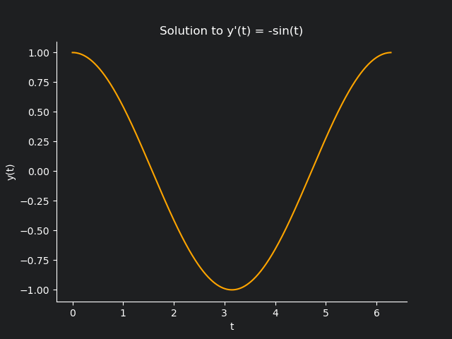
which as we all know is our good ol’ friend $\cos(t)$. Of course, you are more than welcome to change $f$ and obtain numerical solution to any nice function you can think of.
Here is a very nice video on how to approach Dynamic programming problems in general. I also found this walkthrough helpful in illustrating how to structure a good DP code (a well structured code is half debugging done). Finally, I recommend checking out these problems if you want to practice some more.
For now, I will leave you with a couple of exercises to try and play around with for yourself.
Exercises
Exercise 1: In the recursive Fibonacci algorithm without DP, prove that the number of function calls to calculate fib(i) is $F_{n-i+1}$ for all $i \geq 2$.
Exercise 2: What happens in the third DP example if $f$ is discontinuous in the given domain? Say $f$ is piecewise with pieces $f_1$ in $[0,T_1)$ and $f_2$ in $[T_1, T_2]$. Does the solution $y(t)$ looks like it would converge to the piecewise function with pieces $y_1$ in $[0,T_1)$ and $y_2$ in $[T_1, T_2]$ ? If so, can you prove this mathematically?
Exercise 3: Construct the first $n$ terms of the Newman-Conway sequence defined as
$$P(n) = P(P(n-1)) + P(n-P(n - 1))$$
where $P(1)=P(2)=1$.
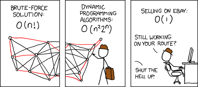
As a reward for making through this blog post, here is a funny cartoon from xkcd (funny if and only if you are familiar with the travelling salesman problem.)
- 1.I did not actually wait for the answer, I lost patience after 10 minutes. ↩