L-systems and generalized fractal generation
This post is the promised follow up to my previous post Everything is $\aleph_1$. In the previous post, among other things, we considered the following problem:
The cardinality of following pairs of sets are the same: $[0,1]\times[0,1]$ and $[0,1]$
We resolved this problem by taking advantage of the uniqueness of decimal expansion of real numbers (up to ambiguities with infinite trailing 9s, which we took care of). However, this solution was by no means my first approach to this problem. As a matter of fact, the first thing that came to mind when I read the problem was the so called Hilbert’s (space filling) curve (In fact, any space filling curve would work). We will explore Hilbert’s curve, which is kind of a fractal, shortly and show that it indeed works as a valid example in this case. This post, however, is motivated by what came after I proved this claim. You see, once I had such a nice result, I really wanted to write a blog post about it; and having decided to write a blog post about it, I really wanted to animate the space filling nature of Hilbert’s curve (whatever that means). It is this pursuit that led me to this very general procedure to generate fractal like structures by constructing what are called Lindenmayer systems (or L-systems for short).
So in this post, we will first encounter the Hilbert curve, and (visually) verify why it is a solution to the problem at hand. Once we have seen that, we will delve into what L-systems are, and how to perhaps design an engine that would write those systems out and draw the corresponding fractals. Finally I will show off some of the really beautiful fractal creations that the engine made possible. I should also give a huge shout out at this point to Grant Sanderson’s math animation engine, manim, which made possible all the stunning visuals I have in this post.
Hilbert’s curve
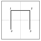
The Hilbert curve $f$ is the uniform limit of a sequence of piece-wise linear curves all contained inside the unit square, with the length of the $n^{th}$ curve $f_n$ being $2^n - 2^{-n}$. The curve itself is produced inductively. The first iterate is obtained by taking the unit square, dividing it into four quadrants and joining the midpoints of the four sub-squares using a piece-wise linear continuous curve as shown below
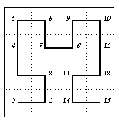
After doing this, each of the four sub-squares are further subdivided into four quadrants of sub-sub-squares. The current curve is removed, and in its place, four copies of the current curve, scaled down by a factor of four, are distributed to each of the sub-sub-squares. The bottom left and right copies are rotated by $90$ and $275$ degrees clockwise respectively before the open ends are connected. The second iterate obtained form the first, is displayed below
And this process proceeds inductively. The sequence of curves and its space filling nature is best illustrated by the following animation1
If we can, for a moment, take for granted that this limiting curve $f$, if it exists, indeed fills the space of the unit square (that is to say, the curve passes through every point on the unit square) then we get our desired (remarkable) result! This is because $f_n$ has length $\ell(n) = 2^n - 2^{-n}$ and in the limit as $n \to \infty$, we have $f_n \to f$ and $\ell(n) \to \infty$. This means, in the limit, we are essentially squeezing all of $\mathbb{R}$ into the unit square2. But we know from part $(a)$ of the same problem (refer previous post) that the cardinality of $[0,1]$ is the same as that of $\mathbb{R}$. Thus, a reparameterization using either $\arctan$ or the other method illustrated in the previous post gives our desired result.
Thus, the only thing that is left to show is that the sequence $\{f_n\}$ uniformly converges to the function $f$ and the function $f$ is has the desired space filling properties. I was originally going to produce my proof of the statement here, but then in trying to figure out some small technicalities that I encountered while writing it up for the blog post, I came across this post on Stack Exchange which has a few slick proofs (from PhoemueX and Martin Argerami) of the statement, that are much better than my ad-hoc constructions and calculations. I will at some point in the future come back to this post and unpack their arguments with visual aid. But for now, let us set our heart at ease and move on to the main star of the post.
L-systems
Context rambling
Having submitted my assignment, and having wanted to write a blog post about the subject – I started my search for a reasonable way to recursively draw the Hilbert curve. After all, this is a textbook example of a recursive process. Of course, as any realistic search goes, my first pit-stop was at Wikipedia to see if there is a recursive closed form functional equation to $f_n$. If I was able to find such a thing (and I am sure someone with infinite patience can figure it out if they set their mind to it) I would hit the jackpot because then all I really had to do was set up manim and tell the compiler what to do, and that was the less contrived bit. But when I went to Wikipedia and looked up the Hilbert curve, lo and behold, there was pseudo-code for generating the fractal! My day was getting better and better!
But then right below the pseudo-code I saw this entryway to a rabbit hole.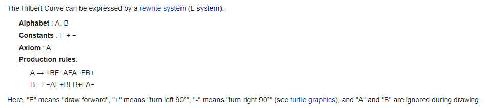
The language seemed weirdly formal for any of the ad-hoc fractal generation I was doing and so I naturally started wondering what an L-system was. Whatever it was, it indeed sounded hella cool. So I started looking into it.
L-system background
L-systems or Lindenmayer systems (named after the biologist who invented the concept whilst studying algae cultures) is a type of string rewriting system. In order the understand what a string rewriting system is, we will start with a set $\Sigma$ of symbols, or alphabets. Then on top of this $\Sigma$ we construct a new set $\Sigma^*$ which is defined to be the smallest set containing $\Sigma$ that also contains all possible finite combination of alphabets in $\Sigma$. That is to say $\Sigma^*$ is the collection of words whose alphabets come from $\Sigma$. Finally for the re-writing part, we consider a binary relation $R$ on $\Sigma^* \times \Sigma^*$. Elements of this relation are denoted $(u \to v)$, and one can essentially understand this as replacing the string $u$ with the string $v$.
L-systems are string rewriting systems but with some more added structure. This additional structure is manifested through the relation $R$, which in this case is called production rule(s) and realized through attaching an extrinsic meaning to certain symbols. It was whilst studying about these L-sytems that I realized that these are precisely the most natural way to generate fractals through code.
This is because while describing in words, how a fractal is constructed, the most natural thing to do is to describe the process iteratively. Say for example, if I were to explain to you how to construct the Cantor set, I would say “Take a line segment of length 1, remove the middle third, for each of the two new line segments, remove their middle thirds, and now to each of the eight line segments, remove their middle thirds and so on and so forth ad infinitum and the resulting set is what the Cantor set is” and you would know exactly how to go about drawing successive iterations of the Cantor set. L-systems basically do exactly that, but in a formal way!
The L-system for the cantor set is given by $\Sigma = \{$A, B$\}$. The initial string (or the axiom) is the word A and the production rules are A $\to$ ABA and B $\to$ BBB. The added structure to these rules are realized when we tell the computer to take the string in the $n^{th}$ step and interpret any A it sees as “draw a line of a specified length” and any B it sees as “move forward by a specified length”. Forgetting these added interpretations for a second, let us just understand the evolution of the axiom A if we treat this process purely from the standpoint of string rewriting.
So the evolution of the axiom tracks as follows:
- A (axiom)
- ABA (The rewriting A $\to$ ABA was performed)
- (ABA)(BBB)(ABA) = ABABBBABA (A $\to$ ABA twice and B $\to$ BBB once)
- ABABBBABABBBBBBBBBABABBBABA (I cant be bothered…)
- …
As we can see, this does get out of control real fast. But now, let us plug back in the interpretation that gives L-systems that added structure. Let us now tell the compiler that in the $n^{th}$ iteration it must understand any $A$ it sees as drawing a horizontal line of length $3^{-n}$ and $B$ as moving forward by a length of $3^{-n}$. So, in the $n^{th}$ step, as the compiler reads the string, if it encounters $A$, we ask it to call the function $\mathtt{draw(length)}$ that draws a line of specified length, and if it encounters a $B$, then we call $\mathtt{skip(length)}$ which skips forward by a specified length. Now we reinterpret each of the evolutionary stages above with these function calls
- A $\iff$ $\mathtt{draw(1)}$.
- ABA $\iff$ $\mathtt{draw(1/3)}$, $\mathtt{skip(1/3)}$, $\mathtt{draw(1/3)}$
- ABABBBABA $\iff$ $\mathtt{draw(1/3)}$, $\mathtt{skip(1/3)}$, $\mathtt{draw(1/3)}$, $\mathtt{skip(1/3)}$, $\dots$, $\mathtt{draw(1/3)}$
- $\dots$
The following is a (5-iteration) visual of the compiler doing exactly that!
That is to say, encoded in the word generated by the string rewriting system are the rules to draw the fractal that we started off wanting to describe! In fact, this way of making the compiler understand what we want it to do, is very reminiscent of me explaining in words what I want you to do when I ask you to draw the Cantor set.
While the cantor set is one of the simpler fractals to draw, it is possible to extend this humble idea to any other complicated fractal! In fact, the wiki for L-system provides the rules for a number of basic fractals! The standard set of alphabets are A and B (or sometimes F, G) in addition to which there are also $+$ and $-$ which tell the compiler to rotate in a given direction by a specified angle. In some rare cases, there is one other alphabet that stands for “do nothing”. This opens up a new realm of possibilities. If we could get our hands on the production rules and the axioms for a given desired fractal, then it should be possible to draw that fractal without writing any ad-hoc very specialized code. We could build a fractal engine!
Building an engine
Posted below is a code snippet of the engine I built to generate new rules and then draw the interpretation of the generated rules. This engine is equipped with the standard set of interpretations.
1 | class LSystem: |
All relevant code can be found in my Github.
Animations
Now equipped with the production rules for various beautiful fractals, and this engine, all I had to do is hook this up to manim, make the data compatible across the two platforms and generate some beautiful animations to show off in my blog. Let’s be honest, as cool as this blog post was, you and I both know that we are here to see cool animations of pretty things. So I won’t torture you any further with words.
Here are some animations of fractals evolving through their iterations
The Gosper curve (or flow snake):
The (Arrowhead) Sirpinsky triangle:
The Hilbert curve
The Koch snowflake
In addition to these evolutions, here are some more fractals that are drawn out
Gosper low-resolution ($n$ small):
Gosper high-resolution ($n$ high):
Arrowhead Sirpinsky:
Hilbert curve:
Partial snowflake:
Dragon curve (The prettiest one in my opinion):
- 1.In the animation, the top copies are rotated because $y$-axis runs top-down in the Python canvas. ↩
- 2.Technially we never explicitly squeeze all of $\mathbb{R}$ into the unit square, just larger and larger chunks of it.