Topological Data Analysis - Part 1 - Persistence Barcodes

Arun Suresh

(Last updated: 2025-01-18)

Research, TDA

What is this and why should you care?

This is the first post in a three-part series introducing persistence barcodes in Topological Data Analysis (TDA) and showcasing their use in classifying 3D shapes. These posts are based on answers from my comprehensive exams. TDA, as the tagline goes, seeks to understand the shape of data by analyzing topological features, such as “holes,” to reveal its structure and inform modeling approaches.

This idea is intuitive: our brains subconsciously use topology information to classify numbers. Consider the example of hand-written digits from the MNIST database: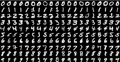

Consider the row of “8”s and note that we can identify the digit “8” by recognizing the presence of two loops, a topological feature unique to that number. However, considering digits like “6,” “9,” and “0” it is clear that we require topology used in conjunction with metric information (eg: where the loop is) to achieve proper classification. This yields the following conundrum: The topological properties express extremely concisely the underlying shape of our data leading to considerable dimension reduction, but it tends to oversimplify models since various non-equivalent shapes (eg: $6$, $9$) might nevertheless be homeomorphic (can be morphed from one to another in a nice continuous way). So even if we could somehow quantify the topological information of a given image as a vector, it is clear that abandoning the (metric properties of the) underlying data in favor of only the topological features is bound to yield subpar results. Thus there is a balance to be struck and a decent bit of topological data analysis as it is applied to real world data involves understanding where this balance lies in a given application.

In this series:
1. Part 1 will focus on defining the the notion of a persistence barcode of an abstract simplicial complex (ASC), and understanding how barcodes extract the topological features of the underlying ASC.
2. Part 2 explores constructing asbtract simplicial complexes from data point clouds which preserves the underlying topological properties.
3. Part 3 implements a classifier for 3D shapes, reducing input feature size by 90% compared to standard methods while achieving comparable performance.

What is an abstract simplicial complex?

We begin with a rather high-brow result from algebraic topology that motivates the study of simplicial complexes in the context of this post.

Every smooth manifold admits a triangulation.

Why is this relevant? A central problem in data science is to estimate a function $f:\mathbb{R}^m \to \mathbb{R}^n$ such that the observed data points lie in the image of $f$ (upto some noise $\epsilon$). A very common assumption that is made is that this estimator $f$ is smooth, and as such it’s image, which is a manifold, is also smooth. The key result now tells us that all of these manifolds are homeomorphic to a space (a simplicial complex) that is built out of triangles and higher dimensional triangles, called simplices. As such all the topological properties of the manifold that estimates our data can be purely understood by studying the simplicial complex that it is homeomorphic to. A simple example of a simplicial complex in three dimension is the tetrahedron

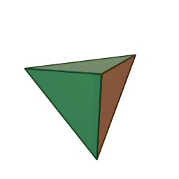
Viewing the tetrahedron as a simplicial complex is to consider the following data: $\Delta = $ 1 tetrahedron $\supset$ 4 triangles $\supset$ 6 edges $\supset$ 4 vertices. We call the (two-dimensional) triangles as $2-$simplices, the edges as $1-$simplices and the vertices as $0-$simplices of $\Delta$.

Here is a more general definition of an abstract simplicial complex:

Definition: An abstract simplicial complex is a pair $\Delta = (V,\Sigma)$ where $V$ is a finite set called the vertex set and $\Sigma$ is a family of non-empty subsets of $V$ such that if $\sigma \in \Sigma$ and $\varnothing \neq \tau \subseteq \sigma$ then $\tau \in \Sigma$ also. The elements of $\Sigma$ are called simplices.

Note: The collection $\Sigma$ decomposes as a disjoint union $\coprod_{k\geq 0} \Sigma_k$ where $\Sigma_k$ denotes the subsets of cardinality $k+1$. That is to say $\Sigma_k$ contains the $k$-dimensional sub-simplices of $\Delta$.

Sanity Check: Apply this definition to the tetrahedron example and identify $\Sigma_k$ for $k\leq 3$.

Finally, given a simplicial complex $\Delta$, we naturally have a notion of viewing $\Delta$ as a filtered simplicial complex by considering subcomplexes as complexes in their own merit. Thereby for a finite dimensional simplicial complex $\Delta$ we can construct a finite simplicial filtration $$\Delta_1 \subseteq \Delta_2 \subseteq \dots \subseteq \Delta_n = \Delta$$
where $n \leq \dim \Delta$.

$p-$th Homology of $\Delta$

In the interest of reducing notational clutter, we will work over the base field $k = \mathbb{F}_2$, although this construction can be done more generally. Given an abstract simplicial complex $\Delta$, we define the simplicial chain complex $C_*(\Delta)$ by letting $C_p(\Delta)$ be the free $\mathbb{F}_2$ vector space on the set of $p-$simplices of $\Delta$, with the boundary map being given as
$$\partial_p: C_p(\Delta) \to C_{p-1}(\Delta); \qquad \sigma \mapsto \sum_{\substack{\tau \subseteq \sigma \ \sigma \in \Delta_{p-1}}} \tau$$
with the understanding that $\partial_0 = 0$ and $C_p(\Delta) = 0$ for all $p<0$. We note here that over a more general field $k$, the sum in the display appears as an alternating sum (after imposing a partial order on $\Sigma_p$ to determine which $p-$simplex goes first).

More explicitly, $C_*(\Delta)$ is the following diagram:
$$C_*(\Delta) = C_0(\Delta) \xleftarrow{\partial_1} C_1(\Delta) \xleftarrow{\partial_2} \dots \xleftarrow{\partial_{p}} C_p(\Delta) \xleftarrow{\partial_{p+1}} \dots$$
If $\Delta$ is finite dimensional (which it is in virtually every use case), it is clear from the definition of $C_p(\Delta)$ that this diagram has an infinite tail of zeroes (hence has finite length) - since $C_p(\Delta) = 0$ vacuously for all $p > \dim \Delta$.

Here is an example to make all this concrete: Consider a $\Delta$ triangle (empty interior) on the plane with vertices $a$, $b$, and $c$. In this case, $C_0(\Delta) = \mathrm{span}(e_a, e_b, e_c) \cong \mathbb{F}_2^3$ where the basis $e_a$, $e_b$ and $e_c$ correspond to the zero dimensional sub-simplices of $\Delta$; namely the vertices $a$, $b$ and $c$. And $C_1(\Delta) = \mathrm{span}(e_{ab}, e_{bc}, e_{ca}) \cong \mathbb{F}_2^3$ where $e_{ab}$, $e_{bc}$ and $e_{ca}$ correspond to the one dimensional edges of $\Delta$. We finally note that $C_p(\Delta) = 0$ for all $p\geq 2$. So, we have our complex as follows
$$C_*(\Delta): \mathbb{F}_2^3 \xleftarrow{\partial_1} \mathbb{F}_2^3 \leftarrow 0 \leftarrow \dots$$
where $\partial_1(e_{ab}) = a+b$, $\partial_1(e_{ac}) = a+c$ and $\partial_1(e_{bc}) = b+c$. Representing the linear map $\partial_1$ as a matrix we see that it has the following form:
$$\partial_1 = \begin{bmatrix} & (ab) & (ac) & (bc) \\ (a) & 1 & 1 & 0 \\ (b) & 1 & 0 & 1\\ (c) & 0 & 1 & 0
\end{bmatrix}$$
We have a matrix (linear map) - and the first thing we should ask ourselves, is where is this zero? Namely, what is the kernel of $\partial_1$? The computation is fairly standard, and we immediately see that the kernel is one-dimensional, namely $\mathrm{span}([1,1,1]) = e_{ab} + e_{ac} + e_{bc}$. This has a very intuitive meaning! If we interpret the sums in $C_p(\Delta)$ as being “unions” of $p-$faces in $\Delta$, then this element precisely captures a cycle of $1-$faces in $\Delta$, and moreover this is also saying that this cycle is not a boundary of anything (evaluates to zero under the boundary map) - identifying the topological feature of having a “hole” in the middle of our triangle.

More generally, we note a crucial property of $\partial_p$ in the following proposition

Proposition 1: Given vector spaces $C_p(\Delta)$ as above, we have $\partial_{p}\circ \partial_{p+1} = 0$

See footnote¹ for proof. Proposition 1 gives rise to a very important consequence - namely that $\mathrm{im}(\partial_{p+1}) \subseteq \ker(\partial_{p})$. This leads to our main definition

Definition: For any integer $p \geq 1$, the $p-$th homology of a simplicial complex $\Delta$ is the quotient vector space
$$H_p(\Delta) = \frac{\ker(\partial_{p})}{\mathrm{im}(\partial_{p+1})}$$
The dimension $\beta_p(\Delta)$ of $H_p(\Delta)$ is the $p-$th Betti number of $\Delta$, and is simply given as $\dim \ker(\partial_{p}) - \dim \mathrm{im}(\partial_{p+1})$.

The elements of $\mathrm{im}(\partial_{p+1})$ are called $p-$boundaries and the elements of $\ker(\partial_{p})$ are called $p-$cycles. Intuitively, $p-$cycles that are not $p-$boundaries represent $p$ dimensional holes, and as such we can understand $\beta_p$ as counting exactly the number of $p-$dimensional holes in $\Delta$.

2. Functorality of $H_p(-)$

This section establishes a very important abstract property of homology, which captures the fact that if we are given a map between two simplicial complexes $\Delta$ and $\Delta’$ – we can construct a very natural map between the $p-$dimensional homologies of the two complexes. This gives us a recipie to take a map of simplicial complexes and understand concretely how the topological features of the source complex change under application of the simplicial map. This is made precise below:

We begin by noting that if $\phi: \Delta \to \Delta’$ be a map of simplicial complexes, then there is an induced $\mathbb{F}_2$ linear map $\phi_p: C_p(\Delta) \to C_p(\Delta’)$ defined as
$$\sum_{\sigma \in \Delta_p} c_{\sigma}\sigma \mapsto \sum_{\substack{\sigma \in \Delta_p \ \phi(\sigma) \in \Delta_p’}} c_{\sigma}\phi(\sigma)$$
for any $p \geq 0$ and $c_\sigma \in \mathbb{F}_2$. This definition yields the following crucial proposition

Proposition 2: We have the following commutative diagram

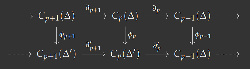
and hence, we have induced maps $\tilde{\phi}_p: H_p(\Delta) \to H_p(\Delta’)$ given by $[c] \mapsto [\phi_p(c)]$.

See footnote² for proof.

Consequently, it is easy to check that given a pair of composable maps $f: \Delta \to \Delta’$ and $g: \Delta’ \to \Delta’’$, then we have equality $\widetilde{(f\circ g)}_p = \tilde{g}_p \circ \tilde{f}_p$, thereby giving us the desired functoriality of $H_p(-)$. That is to say, a map of simplicial complexes induces a map of homologies that is compatible with compositions.

3. Persistence vector spaces

We first make the following general definition:

Definition: A persistence vector space over $k=\mathbb{F}_2$ is a is simply a direct system of $\mathbb{F}_2-$vector spaces indexed by a poset $T$. That is to say, it is a family of $\mathbb{F}_2$ vector spaces {$V_r$}$_{r\in T}$ with prescribed linear maps $\mu_{rr’}:V_r \to V_{r’}$ for each $r\leq r’$ such that $\mu_{r’r’’}\circ \mu_{rr’} = \mu_{rr’’}$ for all $r\leq r’\leq r’’$ (and $\mu_{rr} = \mathrm{id}$).

Now let $\Delta$ be a finite filtered simplicial complex given by the filtration $\Delta_1 \subset \Delta_2 \subset \dots \subset \Delta_n = \Delta$. Now, suppose $1\leq i\leq j\leq n$ and notice that we can apply the $p-$th homology functor to each inclusion $\Delta_i \hookrightarrow \Delta_j$ to get induced maps $\tilde{\phi}_{ij}:H_p(\Delta_i) \to H_p(\Delta_j)$. Moreover, by functorality of $H_p(-)$, we get the following identies: $\tilde{\phi}_{jk}\tilde{\phi}_{ij} = \tilde{\phi}_{ik}$ and $\tilde{\phi}_{ii} = \mathrm{id}$. This observation leads to the following obvious proposition:

Proposition 3: Given a filtered simplicial complex $\Delta$ with filtration $\Delta_1\subset \Delta_2 \subset \dots \subset \Delta_n = \Delta$, then the family ${H_p(\Delta_i)}_{1\leq i \leq l}$ alongside prescribed linear maps $\tilde{\phi}_{ij}$ forms a persistence vector space. We will call this vector space the $p-$th persistence homology of $\Delta$.

The proof is clear from the discussion above. Before we proceed with computing the barcode of persistence vector spaces, we need to impose some finiteness conditions to our persistence spaces. To this end, we make the following definition, and observe its consequences for $H_p(\Delta)$ where $\Delta$ is a filtered simplicial complex.

Definition: We say that a persistence vector space is of finite type if for each $r\in T$, we have that $V_r$ is finite dimensional, and also that there exists some $n \in T$ such that for each $r \geq n$ we have that $\mu_{r,r+1}$ is an isomorphism

This definition applies directly to our situation. Certainly if $\Delta$ is a simplicial complex with a finite filtration with each subcomplex being finite dimensional, then applying the homology functor $H_p(-)$ to the factors we get a direct sum of finite dimensional vector spaces that stabilize. In other words ${H_p(\Delta_i)}$ forms a persistence vector space of finite type.

4. Persistence vector spaces as finitely generated $\mathbb{F}_2[t]$ modules

This part is a bit abstract - but ultimately the underlying core idea of what we are tyring to achieve is as follows: Given a filtered simplicial complex $\Delta_1 \subseteq \dots \subseteq \Delta_n = \Delta$, we first apply the homology functor to get a sequence of maps in homologies. Given these maps, we would like to understand where basis vectors of $H_p(\Delta_i)$ goes as we apply successive $\tilde{\phi}_{i-}$ maps. Tracking how far a basis vector persists (before it maps to 0 in some $H_p(\Delta_j)$ with $j>i$) will inform us how prominent the topological feature represented by the basis vector is in the underlying simplicial complex $\Delta$.

Tracking all these basis vectors for each $i$ is a messy process (and typically computationally expensive). What this section is trying to do is a crucial translation - which says that any persistence vector space precisely corresponds to a “module” over the ring $\mathbb{F}_2[t]$ of all univariate polynomials with coefficients in $\mathbb{F}_2$. A module is generally thought of as the equivalent notion of vector space but now the space is generated over a ring (as opposed to a field). The reason we want to make this translation because there is a very natural way to interpret the birth and death of elements when we work over polynomial rings because of a very deep theorem that characterizes the structure of a modules over a univariate polynomial ring. The more precise details are presented below.

We begin in a more general setting by considering a ring $R$ and noting that there is a natural functor $F$ from the category of direct systems of $R-$modules to the category of non-negatively graded $R[t]-$modules. More precisely, the functor $F$ acts as follows:
$$F({M_i}) = \bigoplus_{i=0}^\infty M_i$$
where elements of $r$ act component-wise, and $t$ acts by shifting the elements of $M_i$ via the structure maps $\mu_{i,i+1}$. More precisely, we have
$$t(m_0,m_1,m_2\dots) = (0, \mu_{01}(m_0), \mu_{12}(m_2), \dots)$$
As for the morphisms, the natural choice is to let $F$ take a morphism $\psi = {\psi_i}: {M_i} \to {N_i}$ of direct systems and send it to the graded map $F(\psi) = \oplus_i (\psi_i): \oplus_i M_i \to \oplus_i N_i$. This choice is certainly compatible with the action of $R[t]$ (by definition of $\psi$) making $F(\psi)$ a graded $R[t]-$module map. Thus $F$ genuinely does form a functor. But, in fact, $F$ does more than just being a functor, as is illustrated by the following proposition.

Proposition 4: The functor $F$ induces an equivalence of categories between the category of direct system of $R-$modules of finite type and the category of finitely generated non-negatively graded $R[t]$ modules.

We skip the formal (categorical) proof of this proposition, but the heart of the argument is contained in Lemma 10.8 of the commutative algebra text by Atiyah and Macdonald, which says:

Lemma 10.8: Let $A$ be a Noetherian ring and $M$ a finitely generated $A-$module with filtration ${M_n}$. Then the following are equivalent:
1. $M^* = \oplus_i M_i$ is a finitely generated $A^* = A[x]$ module
2. The filtration ${M_n}$ is stable.

Returning to our particular application, we let $R = \mathbb{F}_2$. Thus $R[t]$ into a PID, and we interpret Proposition 4 as saying that a persistence vector space uniquely corresponds to a graded module over the PID $R[t]$.

5. Computing the barcode of persistence homologies

We continue letting $R=\mathbb{F}_2$. Given the observation above, we can use the structure theorem for finitely generated graded modules over a graded PID, to see that every such finitely generated module over $R[t]$ must be isomorphic to a direct sum of the form
$$\left(\bigoplus_{i=1}^n \Sigma^{\alpha_i} R[t]\right) \oplus \left( \bigoplus_{j=1}^m \Sigma^{\gamma_j} R[t]/(t^{n_j})\right)$$
where $t^{n_j}$ divides $t^{n_{j+1}}$ and $\Sigma$ denotes a shift in grading.

Finally, we are ready to outline the procedure of obtaining barcodes from persistence homologies. Let a $\mathcal{P}-$interval be a pair $(i,j)$ with $0\leq i < j \leq \infty$. Given a filtered simplicial complex, we construct the $p-$th persistence homology ${H_p(\Delta_i)}$, identify it with a module over the PID $R[t]$ that is isomorphic to a direct sum of the form illustrated in the display above. Now we associate $\mathcal{P}-$intervals to our persistence homology as follows: a (free) summand of the form $\Sigma^{\alpha} R[t]$ corresponds to the $\mathcal{P}-$interval $(a, \infty)$, while a (torsion) summand of the form $\Sigma^{\beta} R[t]/(t^n)$ corresponds to the $\mathcal{P}-$interval $(\beta, \beta+n)$. This association is clearly a bijection. The collection of all these $\mathcal{P}-$intervals constitute the barcode of our persistence homology. We could interpret it as follows: A $\mathcal{P}-$interval $(i,j)$ describes a cycle that is “born” at filtration level $i$ and specifies a homology class until it is annihilated (becomes a boundary) at filtration level $j$.

Ultimately this general theorem gives us a way to just “read off” the birth and death times of certain topological features just by writing our persistence homologies in the special form guaranteed by the structure theorem (and there is an algorithmic process to achieve this representation), thereby bypassing any need to track how basis vectors evolve as we move up our simplicial filtration!

Ending remarks

This is probably the most abstract (and the longest) of the three parts in this series. Kudos for following through! Here is a meme

In part (2) we will discuss ways to construct simplicial complexes from underlying data. See you there!

Proofs

1.Proof of Propositon 1 Given $\sigma \in C_p(\Delta)$, we see that $\partial_{p-1}\partial_p(\Delta)$ is an $\mathbb{F}_2$ linear combination of $p-2$ simplices in $\Delta$. That is $$\partial_{p-1}\partial_{p}(\sigma) = \sum_{\substack{\tau \subseteq \sigma, \ \tau \in \Delta_{p-2}}} \tau.$$ Now note that any $p-2$ subcomplex $\tau$ of $\sigma$ can be obtained from $\sigma$ by deleting two vertices, say $v_1$ and $v_2$. More importantly, this subcomplex $\tau$ can be obtained in two different ways: one by deleting $v_1$ first before deleting $v_2$, and another by deleting $v_2$ first, before deleting $v_1$. Therefore, we see that the face $\tau$ appears twice in the final sum. Since we are working over $\mathbb{F}_2$, we are done. ↩
2. Proof of Proposition 2 Let $\sigma \in C_{p+1}(\Delta)$ be defined by vertices $[v_1,\dots, v_{p+1}]$. We proceed by cases:
Case 1: Say ${\phi(v_i)}$ are all distinct, which in turn tells us that $\phi_{p+1}(\sigma) = [\phi(v_1), \dots, \phi(v_{p+1})] \in C_{p+1}(\Delta')$. Applying the boundary operator $\partial_{p+1}'$ we have $$\partial_{p+1}'\phi_{p+1} (\sigma) = \sum_{j=1}^{p+1} [\phi(v_1), \dots, \widehat{\phi(v_j)}, \dots, \phi(v_{p+1})]$$ which is precisely $\phi_p \partial_{p+1}$ since all the $\phi(v_i)$ are unique.

Case 2: Say $\phi(\sigma) \in C_j(\Delta')$ with $j < p$. In this case, $\partial_{p+1}'\phi_{p+1} = \partial_{p+1}'(0) = 0$. Now for the other direction, say $\sigma = [v_1,\dots, v_{p+1}]$. From our assumption, we know that there are (WLOG) $v_1, v_2, v_3$ such that $\phi(v_1) = \phi(v_2) = \phi(v_3)$. Thus each summand of $\partial_{p+1}(\sigma)$ will contain vertices $v_i$ and $v_j$ with $i,j \in {1,2,3}$. As such, after applying $\phi_{p}$ each summand of the resulting sum defines a sub-simplex of dimension at most $p-1$, and therefore $\phi_p\partial_{p+1}(\sigma) = 0$.

Case 3: Say $\phi(\sigma) \in C_p(\Delta')$. In this case, we still have $\partial_{p+1}'\phi_{p+1} = 0$. For the other direction, say $\sigma = [v_1,\dots, v_{p+1}]$. From our assumption, we know that there must exist exactly two vertices (WLOG) $v_1, v_2$ such that $\phi(v_1)= \phi(v_2)$. Thus applying the boundary operator $\partial_{p+1}$ to $\sigma$, we see the following sum $$\partial_{p+1}(\sigma) = [v_1, v_3, \dots, v_{p+1}] + [v_2, v_3, \dots, v_{p+1}] + \sum_{\tau} \tau$$ where each summand $\tau$ contains both vertices $v_1$ and $v_2$. Upon applying $\phi_p$ to this display, we see that each summand $\tau$ maps to zero since $\phi(\tau)$ is a $p-1$ simplex. On the other hand, the first two $p-$faces evaluate to the same quantity. Since we are working over $\mathbb{F}_2$, we are done!

Finally, to see that the induced map $\tilde{\phi}_p:H_p(\Delta) \to H_{p}(\Delta')$ is well-defined, we do a simple diagram chase. More precisely, we see that if $c \in \ker(\partial_p)$, then it certainly maps to $0$ under $\phi_{p-1}$. By the above commutativity of the square, it must be that $\phi_{p}(c)$ must map to $0$ under $\partial_p'$. Thus $\phi_p(c) \in \ker(\partial_p')$. To show that this map is well defined, we take a different representative $c + c'$ with $c' \in \mathrm{im}(\partial_{p+1})$. Under $\phi_p$, this maps to $\phi_p(c+c') = \phi_p(c) + \phi_p(c')$. Now since $c' \in \mathrm{im}(\partial_{p+1})$, there exists $c'' \in C_{p+1}(\Delta)$ such that $\partial_{p+1}(c'') = c'$. By the commutativity of the diagram once again, we must have that $\phi_{p+1}(c'')$ maps to $\phi_p(c')$ telling us that $\phi_p(c)$ and $\phi_p(c+c')$ are equal upto an element of $\mathrm{im}(\partial'_{p+1})$.
↩