Topological Data Analysis - Part 2 - $\Delta$ from Data.
Recap and introduction
In the previous post we encountered the notion of a barcode of a simplicial complex as a way to capture it’s topological features. From a data science stand point, this was motivated by the fact that any smooth manifold (that we typically expect to model our data) is homeomorphic to a simplicial complex that is built out of higher dimensional analogues of triangles, called simplices. By considering sub-complexes of a simplicial complex, we can naturally filter a finite dimensional simplicial complex into a finite filtration: $\Delta_1 \subseteq \Delta_2 \subseteq \dots \subseteq \Delta$.
In this post, we will discuss some standard ways how we can build a simplicial complex from a finite collection of data points $\mathcal{X}$ in $\mathbb{R}^n$ (or any metric space for that matter). To this end, suppose that we are given a finite data point $\mathcal{X} \subseteq \mathbb{R}^n$.
The Čech complex of $\mathcal{X}$
Fix a parameter $r \in \mathbb{R}$. The Čech complex $Č_r(\mathcal{X})$ at parameter level $r$ is constructed as follows:
1. Each point $x\in \mathcal{X}$ constitute the vertices of the Čech complex
2. Now consdier $B(x, r)$ for each $x \in \mathbb{X}$.
$\qquad$ a. Any $k-$fold intersection of these balls is a $(k-1)-$simplex of the Čech complex between the corresponding vertices.
That is, there is an edge between Čech vertices $x_1$ and $x_2$ if the balls $B(x_1, r)$ and $B(x_2, r)$ intersect. Similarly three fold intersections correspond to a $2-$simplex (a triangle) between the corresponding three vertices, and so on.
The following diagram makes this process clear: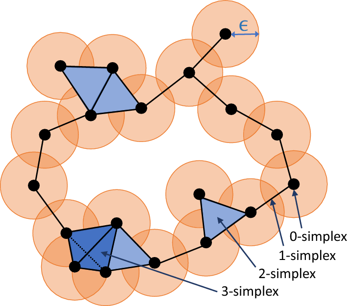
image credit
Notice that if $r_1 < r_2$, then we immediately see that $Č_{r_1}(\mathcal{X}) \subseteq Č_{r_2}(\mathcal{X})$ because if two balls intersect at radius $r_1$ intersect, then they certainly still interesect after “growing” the radius to $r_2$. Moreover, there is also a critical radius $r^* = \mathrm{diam}(\mathcal{X})$1 such that $Č_{r}(\mathcal{X}) = Č_{r^*}(\mathcal{X})$ for all $r>r^*$ since at this level we every ball would pairwise intersect every other ball.
Given a tolerance level $\epsilon$, this gives us a very natural finite filtration of the Čech complex, namely
$$Č_{0}(\mathcal{X}) \subseteq Č_{\epsilon}(\mathcal{X}) \subseteq Č_{2\epsilon}(\mathcal{X}) \subseteq \dots \subseteq Č_{r^*}(\mathcal{X})$$
The Vietoris Rips complex of $\mathcal{X}$
The Čech complex, while extremely intuitive to understand, is computationally messy to compute since it involves determining when two balls intersect, and computing general intersections is a hard computational problem. However, we can take advantage of the fact that these are balls, and cut some corners. This gives rise to the Vietoris complex of $\mathcal{X}$ which is a less refined version of the Čech complex - but is computationally much less expensive.
The Vietoris-Rips $VR_r(\mathcal{X})$ complex at parameter level $r$ is constructed as follows:
1. Consider a non-empty subset $X \subseteq \mathcal{X}$ of cardinality $k \geq 1$
2. Deem that $X$ forms a $(k-1)-$simplex of $VR_r(\mathcal{X})$ if $\mathrm{diam}(X) \leq 2r$
3. Repeat this for all non-empty subsets of $\mathcal{X}$.
Note that at any given parameter level $VR_r(\mathcal{X})$ contains $Č_{r}(\mathcal{X})$, since in Vietoris rips complex it is possible to get a $k-$simplex even without mutual $k-$fold intersection, but it is impossible to obtain that in the Čech complex. Here is an example to illustrate this phenomenon:
Let $\mathcal{X}$ be the vertices of a square of side length $2$. At parameter level $r=1$, the Čech complex gives us the four edges of the square because all four balls of radius 1 are tangential to each other. On the other hand, the VietorisRips complex has additional $2-$simplices because for any vertex $x$, we have it’s two adjacent neighbors $x_1$ and $x_2$ such that $\mathrm{diam}(x,x_1,x_2) \leq 2$ thereby forming a $2-$simplex that is not present in the Čech complex.
Alternatively, here is a pictorial proof: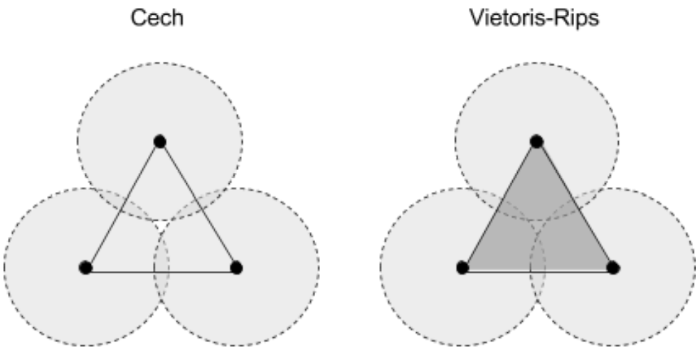
image credit
The above illustrates the sense in which the VR complex is a slightly less refined than the Čech complex. However, calculating pairwise distances is still much easier than checking for interesctions! The VR complex also admits a natural finite filtration much like the Čech complex (given a tolerance level $\epsilon$):
$$VR_0(\mathcal{X}) \subseteq VR_\epsilon(\mathcal{X}) \subseteq VR_{2\epsilon}(\mathcal{X}) \subseteq \dots \subseteq VR_{r^*}(\mathcal{X}).$$
For computational purposes the VR complex remains robust enough. For our classifier implementation in part 3 , we will use the VR complex to build our simplicial filtration.
Delaunay complex of $\mathcal{X}$
– Coming soon –
Alpha Shape complex of $\mathcal{X}$
– Coming soon –
- 1.If $T \subseteq \mathbb{R}^n$ is a finite subset, $\mathrm{diam}(T)$ is the largest distance between any two points of $T$. ↩